Computational Modeling
Valdés-Sosa et al. (2000) introduced a transparent-motion design that has spawned numerous subsequent psychophysical and neurophysiological studies of object-based attention*. Taken together, these studies appear to provide some of the best evidence for object-based selection (Reynolds, Alborzian, & Stoner, 2003; Çatak, Özkan, Kafalıgönül, & Stoner, 2022). Although there are some design differences in the various studies inspired by Valdés-Sosa and colleagues' original study, all of these studies used stimuli composed of two superimposed counter-rotating dot fields. One of the two dot fields is “cued”, either endogenously (e.g., fixation point color indicating the color of the field to be attended if the dots are differently colored) or exogenously (e.g., by a delayed-onset of one dot field, see below). The rotations of the dot fields are interrupted by brief translations (one or two translations, depending upon the design), and subjects are asked to report the direction of those translations. These translations consist of a subset of the dots moving coherently in typically one of eight directions. To discourage tracking of individual dots, the remaining dots of the translating dot field translate in randomly chosen directions. Numerous studies using this basic design have repeatedly found that subjects judge translations of the cued dot field more accurately than translations of the uncued dot field (Khoe et al., 2005; López et al., 2004; Mitchell et al., 2003; Mitchell, Stoner, & Reynolds, 2004; Pinilla et al., 2001; Reynolds et al., 2003; Rodríguez et al., 2002; Stoner & Blanc, 2010; Valdés-Sosa, Cobo, & Pinilla, 2000). Several of these studies also reported electrophysiological (ERP) correlates of the cueing advantage (Valdés-Sosa, Bobes, Rodríguez, & Pinilla, 1998; Pinilla et al., 2001; López, Rodríguez, & Valdés-Sosa, 2004; Rodríguez & Valdés-Sosa, 2006; Çatak et al., 2022).
As observed by Stoner & Blanc (2010), for the object-based account to hold for these experiments, the attentional cue — whether endogenous, exogenous, or both — must first privilege the subset of overlapping dots rotating in one direction and then privilege those same dots when they translate. The visual system must therefore "bind" the cued rotation to the subsequent translation in an object-specific manner. The mechanism of such binding has never been identified, nor has any directly applicable model been advanced. In this section, we first question the need for an object-based account. We demonstrate that established feature-based biased-competition and normalization models appear to account for previous results. We then show that these models cannot, however, account for the results of "feature-swap" experiments devised by Stoner and Blanc. We then consider computational models of incremental complexity that might account for those results as well as other findings attributed to object-based attention in transparent-motion displays.
* The term "surface-based attention" is sometimes used interchangeably in this literature, emphasizing perceptual surfaces rather than discrete objects as the units of selection; the two framings make similar predictions in transparent-motion paradigms.
Non-object-based models
The motion-competition model
In our initial attempts to model "object-based" effects, we will focus on the delayed-onset design introduced by Reynolds, Alborzian, & Stoner (2003), which features a single-translation (Figure 1). As reviewed above, the translation directions of cued (delayed) dot fields are reported more accurately than translations of the uncued dot field. Similarly, translations of the cued dot field yield larger ERPs than translations of the uncued dot field (Çatak et al., 2022). In considering how preferential processing of a cued dot field’s rotation direction might give rise to preferential processing of that dot field’s translation direction, we realized that previous designs suffered from a motion-duration confound that admitted an explanation not requiring object-based selection. This confound applies to both the original “two-translation” design devised by Valdés-Sosa et al. (2000) and to the “delayed-onset” design illustrated in Figure 1. Figure 1B makes this explicit: cued translations always occur alongside the older rotation direction, uncued translations during the newer one.
Stoner and Blanc realized that this confound offered a simpler "motion-competition" explanation that implied that which object (cued/delayed or uncued/undelayed) happens to translate is irrelevant. Specifically, they posited that: 1) owing to neuronal adaptation, neuronal responses to the delayed (newer) rotation direction at the onset of the translation are larger than responses to the non-delayed (older) rotation direction. 2) neurons responding to the continuing rotation direction (i.e. the sole rotation direction present during the brief translation) suppress responses to the translation. As a consequence of these two mechanisms, suppression of the translation responses would be greater when the translation occurred in the presence of the delayed rotation direction. This account predicts that, consistent with experimental results, cued translations would thus evoke larger neuronal responses than uncued translations.
This reframing of the paradigm follows from established competitive interactions among direction-selective neurons (Qian & Andersen, 1994; Snowden, Treue, Erickson, & Andersen, 1991; Krekelberg & Albright, 2005). According to the biased-competition account of attention (Desimone & Duncan, 1995), co-activated populations of neurons compete, and the winner can be tipped by stimulus strength — such as luminance contrast — or by exogenously- or endogenously-directed selective attention (Luck, Chelazzi, Hillyard, & Desimone, 1997; Moran & Desimone, 1985; Reynolds, Chelazzi, & Desimone, 1999). To render these mechanisms concrete, Stoner & Blanc (2010) applied the biased competition model of Reynolds, Chelazzi, & Desimone (1999) to the delayed-onset paradigm.
To make this model as simple as possible, we will approximate the rotations as translations. Figure 2 illustrates why this is a defensible approach: area MT RFs would see rotating dots as translations approximately and their responses to those rotations should be very nearly the same as to pure translations at those locations. This modeling exercise is not dependent on that approximation but it allows us to imagine that our neurons are all MT neurons rather than supposing interactions with area MST or between MT and MST (other cortical areas with directionally-selective neurons could also be involved.)
This local relabeling of the motions yields the feature trajectories shown in Figure 3. Note that these feature trajectories provide two types of information: 1) Feature information. The directions of motion and colors present at any given time. We will discard color information for these early modeling efforts. This is justified by Mitchell et al. (2004)'s demonstration that the cueing effect survives color difference removal. 2) Object identity as defined by dot continuity. For our initial modeling work, we are going to assume that it's only the direction of motion information that's important and hence which object happens to move in which direction is irrelevant. Figure 3 toggles back and forth from illustrations with both object and motion information and just the motion information -- it's the latter that illustrates the input we provide to our models. This is completely consistent with the large RFs of area MT neurons.
The object-neutral view of Figure 3 makes the model's prediction explicit: because the motion swap leaves the directional input unchanged (A and B are identical; C and D are identical), a model driven solely by those signals cannot distinguish the cued no-motion-swap condition from the uncued motion-swap condition, nor the uncued no-motion-swap from the cued motion-swap, and must therefore predict that the cued advantage reverses under a motion swap. Figures 4 and 5 trace the computation in detail; Stoner & Blanc (2010) tested that prediction directly.
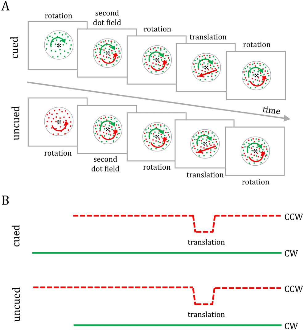
Figure 1. Delayed-onset design (Çatak et al., 2022). (A) One rotating dot field appears followed by the second "delayed" dot field. Two superimposed dot fields rotate in opposite directions around the fixation point, allowing the perception of two transparent surfaces. Following the rotation, either the delayed (cued) or non-delayed (uncued) dot field translates briefly. After the translation, both dot fields continue to rotate. (B) Feature-based illustration of timeline. The two dot fields are differentiated by line style (dashed or solid) and with dot field colors indicated by the line colors. The vertical line placement indicates the different motion directions: clockwise rotation (CW), counter-clockwise rotation (CCW), and translation. The onset differences in this design result in "cued" translations occurring in the presence of the older rotation direction and "uncued" translations occurring in the presence of the newer rotation direction.
Figure and caption reproduced from Çatak, Özkan, Kafalıgönül & Stoner (2022), Cortex 151, 89–104, © Elsevier.
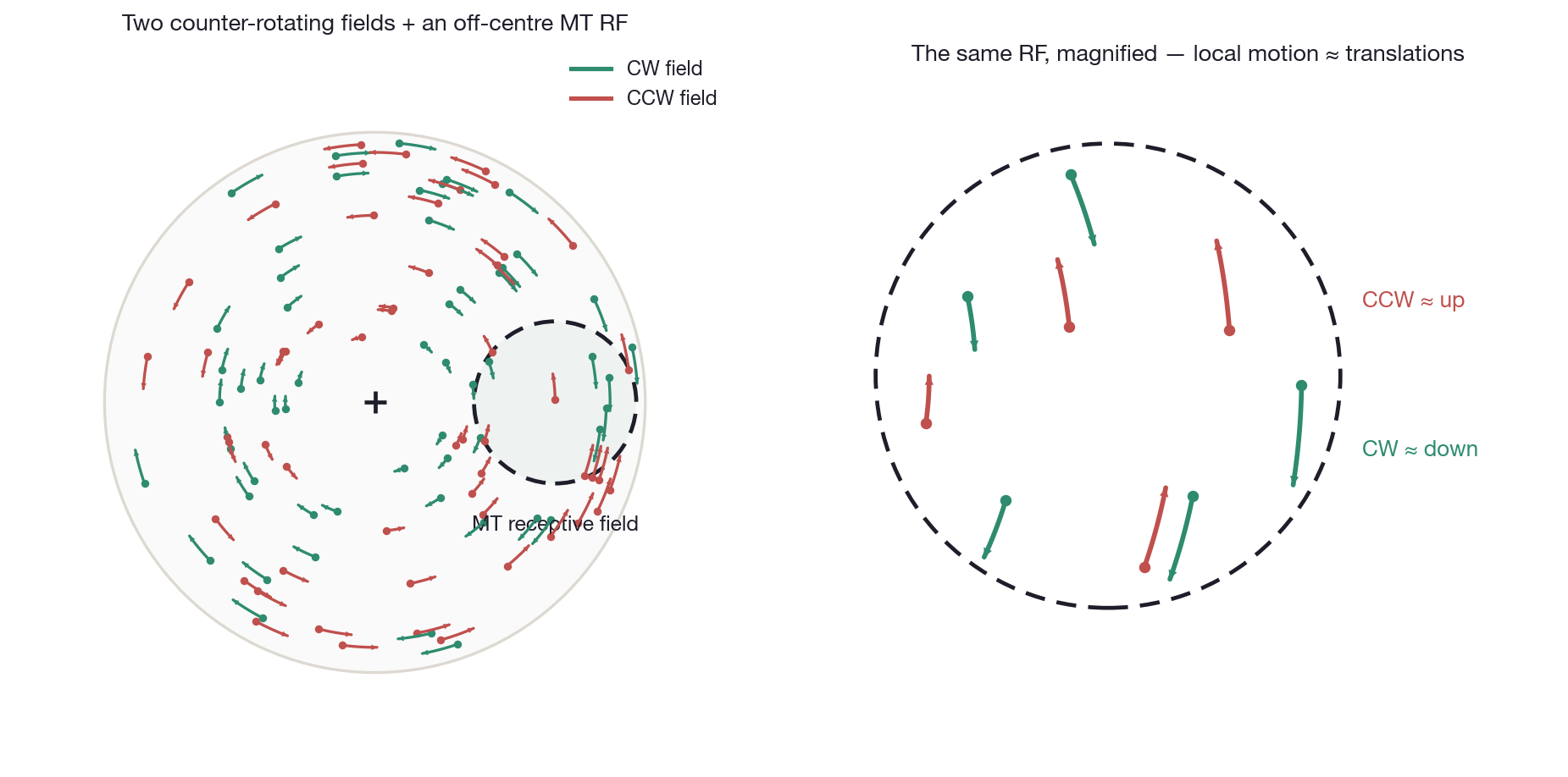
Figure 2. Why we can treat the inputs as translations. MT neurons have large receptive fields that take in both transparent surfaces at once. For a receptive field placed off-center (here directly right of fixation), each rigidly rotating field is, locally, approximately a translation: the clockwise field drifts down and the counter-clockwise field drifts up. The right panel is that same receptive field magnified — the identical dots and their identical rotation arcs, not an idealized patch — so the motions shown are exactly those in the stimulus. (Each trace is 100 ms of motion at the stimulus's 81°/s rotation; dot density is Stoner & Blanc's 5 dots/deg² per field.) So the two rotations and the brief translation can all be represented as motion directions on a single axis — the population drive that feeds the model. V1 supplies that directional signal — its small receptive fields extract the local motion direction most precisely — but V1 is the input, not a model stage: this rotation drive depends on motion direction alone, so it is unchanged by a color or identity swap (the motion swap is taken up in Figure 3). The model's own stages live in MT. Crucially, the model does not depend on this local-translation simplification. It simply lets us reason with a directional MT drive and defer MST and rotation-selective neurons, which can be layered in later.
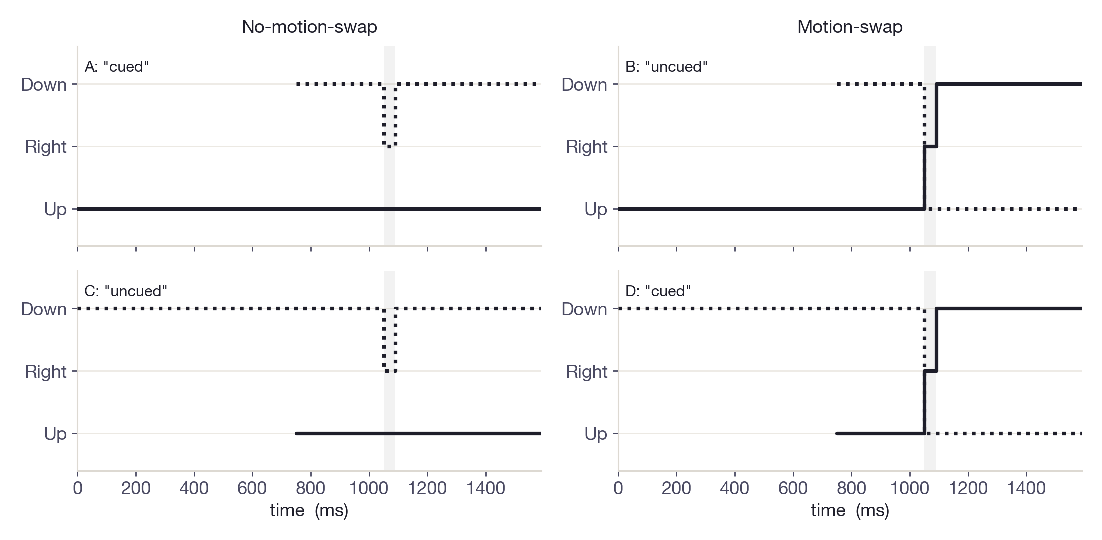
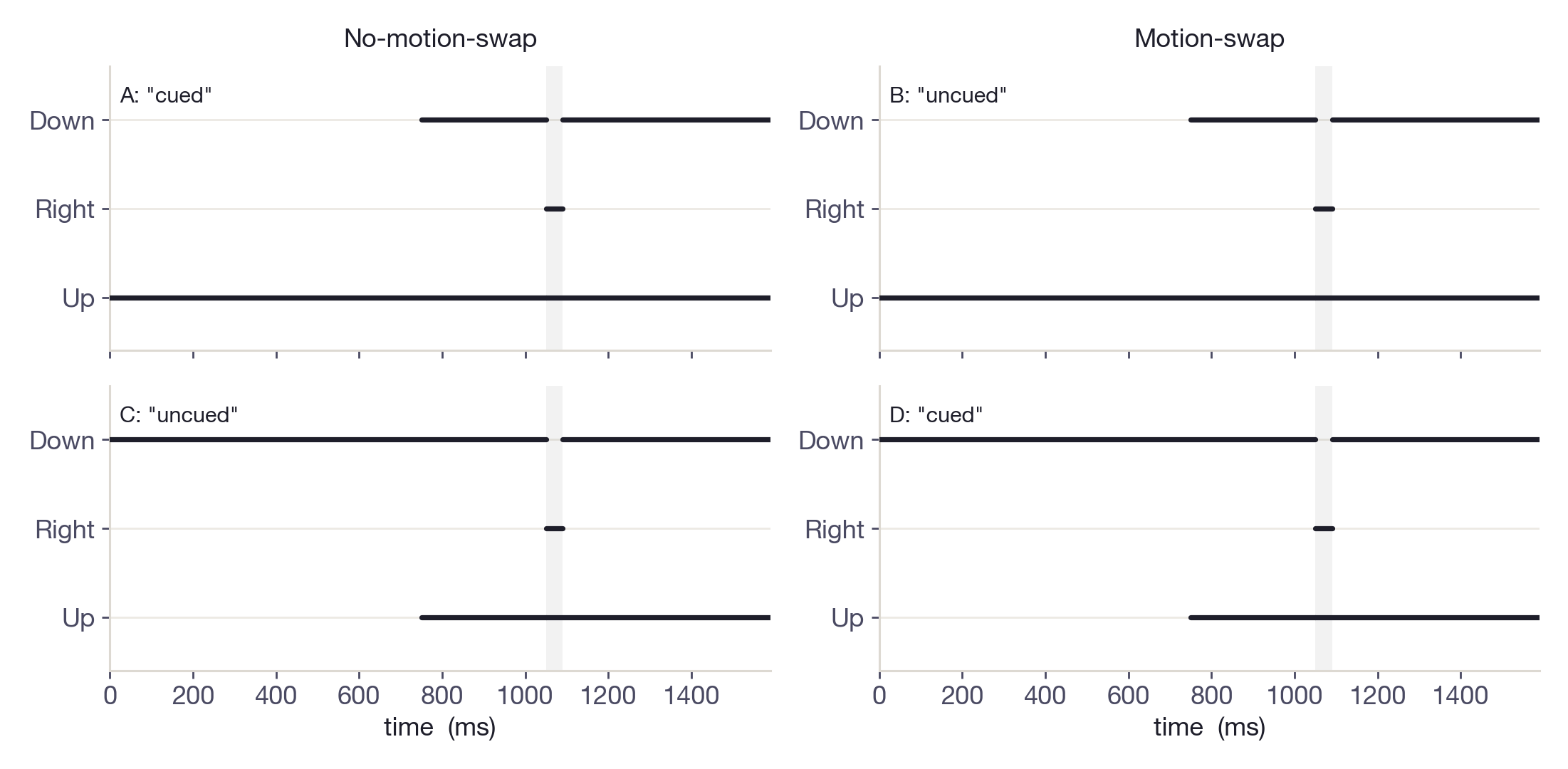
Figure 3. Feature trajectories of no-motion-swap and motion-swap conditions (A–D, after Stoner & Blanc, 2010, Fig. 4). See Figure 1 for stimulus conventions. Within the object-based framework, "cued" indicates that the delayed dot field translates and "uncued" indicates that the non-delayed (first-on) dot field translates. For our modeling exercise, we assume a single MT hypercolumn whose collective receptive field lies on the right side of the rotating display (see Figure 2): within this RF, clockwise rotation is locally downward motion, counter-clockwise rotation is locally upward motion. The brief translation (in this exercise) is rightward. Thus the motion signals within this collective RF are: downward, upward, and rightward. Note that the brief translation also includes a 50% random-direction component. From the point of view of our biased-competition model, these motions are all that matters: which object (dot field) happens to be undergoing those motions is irrelevant (as are the "cued/uncued" labels). Thus, while the object-based depictions retain the line-style differentiation of the two dot fields, the what the model sees depictions show only how the motions evolve over time. From the latter depiction, you see that the cued no-motion-swap condition is identical to the uncued motion-swap condition. Similarly, the uncued no-motion-swap condition is identical to the cued motion-swap condition. Hence, if it's just the motion signals present in the RF (independent of object identity) that determines the cueing effect, the motion-swap manipulation should reverse the cueing effect. Stoner & Blanc (2010) tested that prediction and found that the cueing effect did NOT reverse: the cueing effect was specific to object (dot field) identity, as the object-based framework assumed.
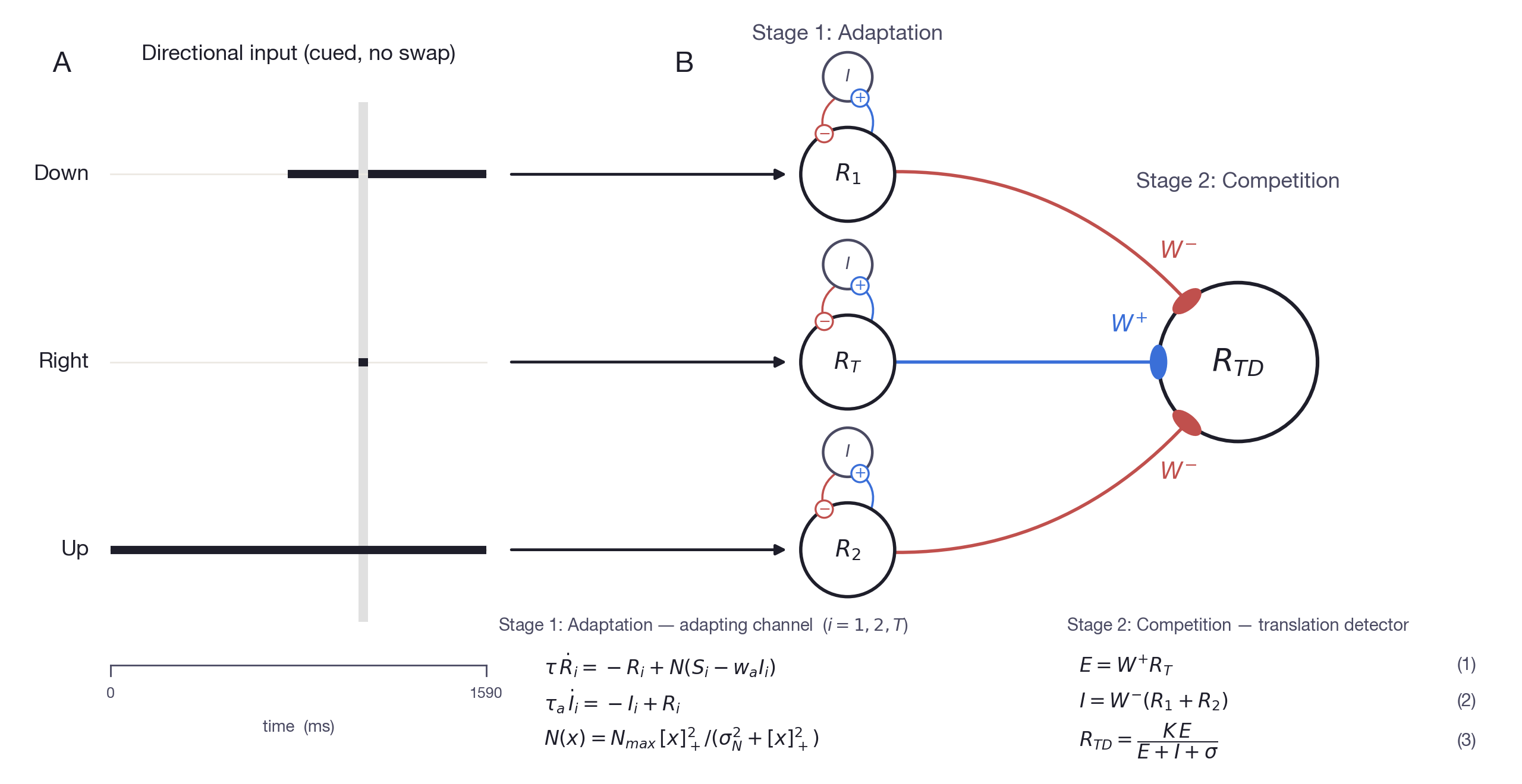
Figure 4. Inputs feeding the biased-competition circuit. (A) The directional time-varying input into the model for a cued, no-swap trial (see Figure 3). (B) The three direction-selective model neurons of "Stage 1" receive this excitatory directional input. We can think of these three neurons as belonging to a single MT hypercolumn (see Figure 2). These three neurons each have a directional preference corresponding to one of the three predominant directions within the collective receptive field of that MT hypercolumn: Down, Right, and Up. The responses of these three Stage 1 neurons adapt over time, mediated by recurrent inhibition from the I unit and modeled by the equations shown. These adapted responses then feed into the Stage 2 translation detector R₍TD₎, with R₍T₎ providing excitatory (W⁺) input and R₁ and R₂ providing inhibitory (W⁻) shunting input. Taken together, these interactions implement the biased-competition computation of Reynolds et al. (1999). In this cued example, Down appears first and is therefore more adapted by translation onset, while Up arrives later. Hence the translation competes with a weaker inhibitory input than occurs with the uncued condition. In our simple model, we take the output of this translation detector as our measure of how well the model detects the translation (see Figure 5).
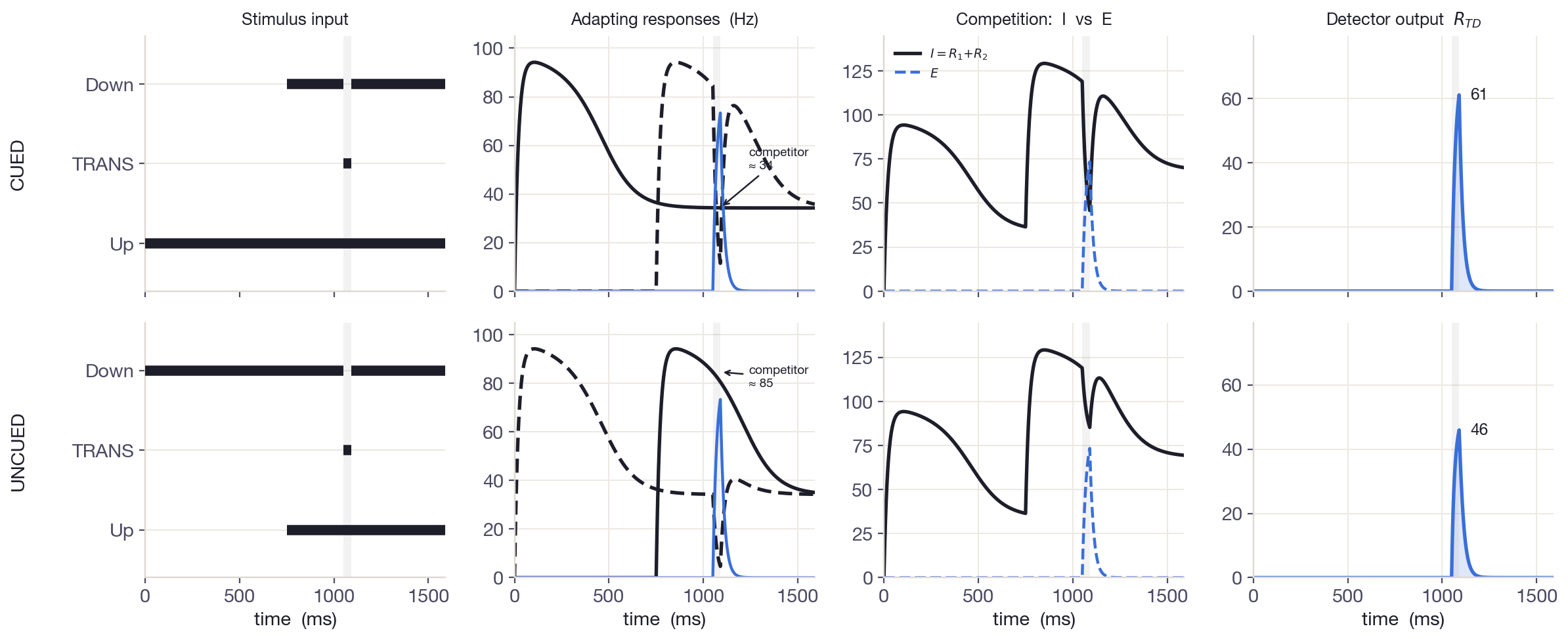
Figure 5. The computation, end to end. Each row is one of the two cases the four trial types collapse to (CUED = the delayed-onset field translates; UNCUED = the first-on field translates — recall A≡B and C≡D at the input). Reading left to right: (1) Stimulus input — the two rotation directions and the brief translation as binary direction channels (solid = CW / first-on field; dashed = CCW / delayed field; the translating field's rotation is interrupted during the window; blue = translation). (2) Adapting responses — the Stage-1 MT direction channels (Eqs 1–3); the delayed field, having had less time to adapt, responds more strongly than the first-on field. (3) Competition — total divisive inhibition I = R₁+R₂ versus excitation E from the translation. During the translation the translating field's rotation is interrupted, so its channel drops out of the inhibitory pool and I notches down; the notch is deeper when the interrupted field is the less-adapted (delayed) one. (4) Detector output R₍TD₎ = KE/(E+I+σ) — E is the same in both rows, so the deeper inhibition notch in CUED yields the higher peak (here 61 vs 46, a +33% bias). Note the directional input (column 1) is identical with or without a feature swap — the swap never enters this cascade.
The normalization model of attention
Reynolds & Heeger (2009) — attention supplies the bias
The competition model produced the cued advantage from adaptation, with no attentional term. Reynolds & Heeger (2009) describe a normalization model of the same biased-competition family in which the bias instead comes from attention: an attention field multiplicatively scales the neurons tuned to the attended stimulus, before divisive normalization. Running that model on the very same delayed-onset stimulus — with a fixed attentional gain on the cued direction standing in for Stoner & Blanc's adaptation — reproduces the cued advantage. The two accounts are, at this level, interchangeable: whether the cueing bias is supplied by adaptation or by attention, the normalization stage turns it into the same response difference.
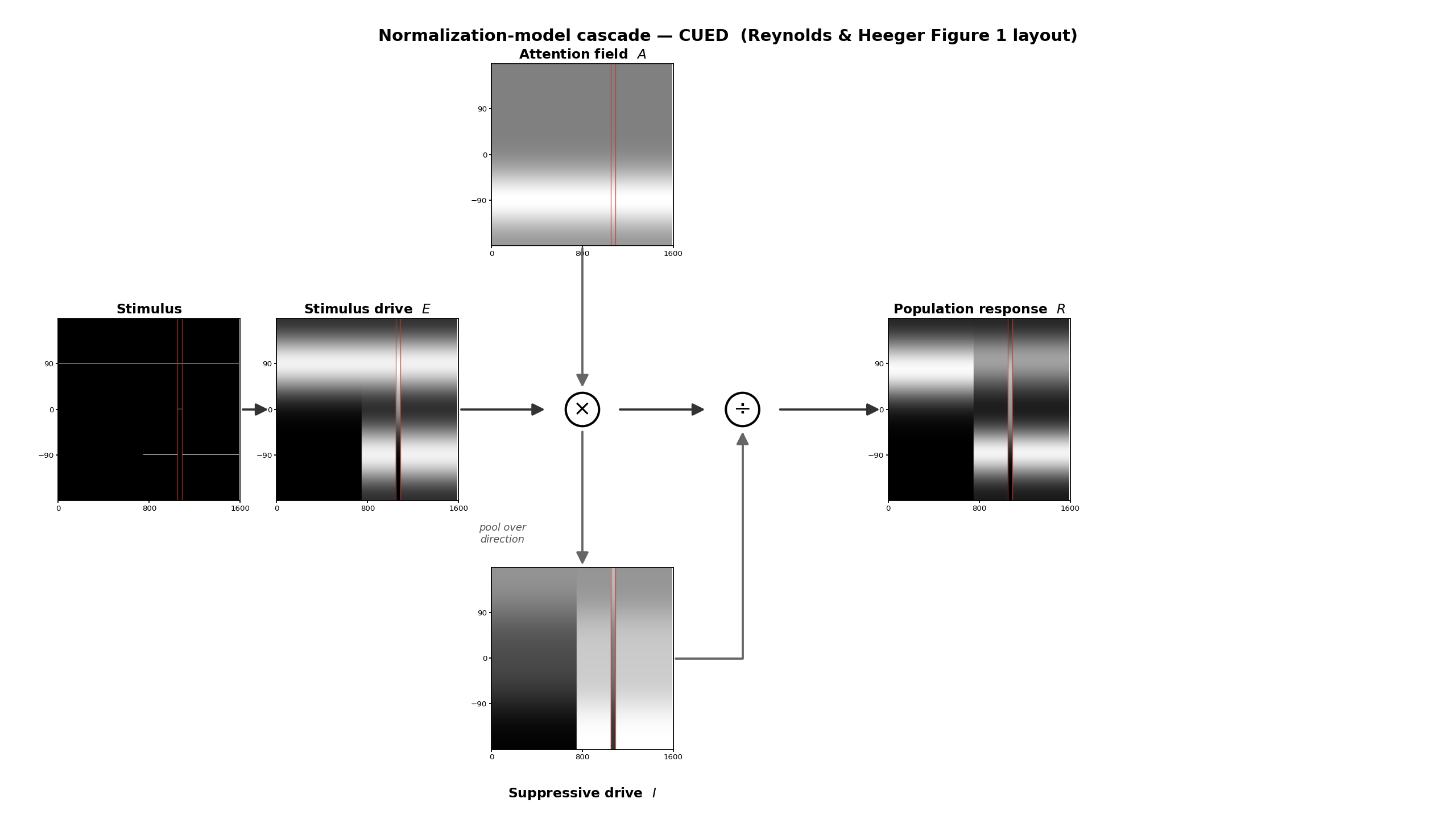
Figure 6. The normalization model on the same stimulus (Reynolds & Heeger Figure 1 layout). R&H's model written as their Figure-1 visual equation, computed with a bit-for-bit verified port of their `attentionModel.m`: the stimulus drives a direction-tuned stimulus drive E, which is multiplied (×) by the attention field A(θ) — a fixed gain bump on the cued (Down / −90°) direction — and the product E·A is then divided by the suppressive drive I to give the population response R = (E·A) / (I + σ). The suppressive drive is that same product, pooled — I = (E·A) ⊛ (Iₓ ⊗ I_θ) — so the attention field shapes both the numerator and (through the pool) the denominator. Each panel is a grayscale map over preferred motion direction (vertical) and time (horizontal); white = high (following R&H, where midgray = 1 and white > 1). The suppressive drive is present throughout the trial — wherever the rotations drive the population — not a translation-only term. The attention field replaces Stoner & Blanc's adaptation as the source of bias. Axes, kernels, and normalization are R&H's, with time substituted for their spatial receptive-field axis (σ = 10⁻⁶) — see the note below Figure 7 on exactly what that substitution does and does not change.
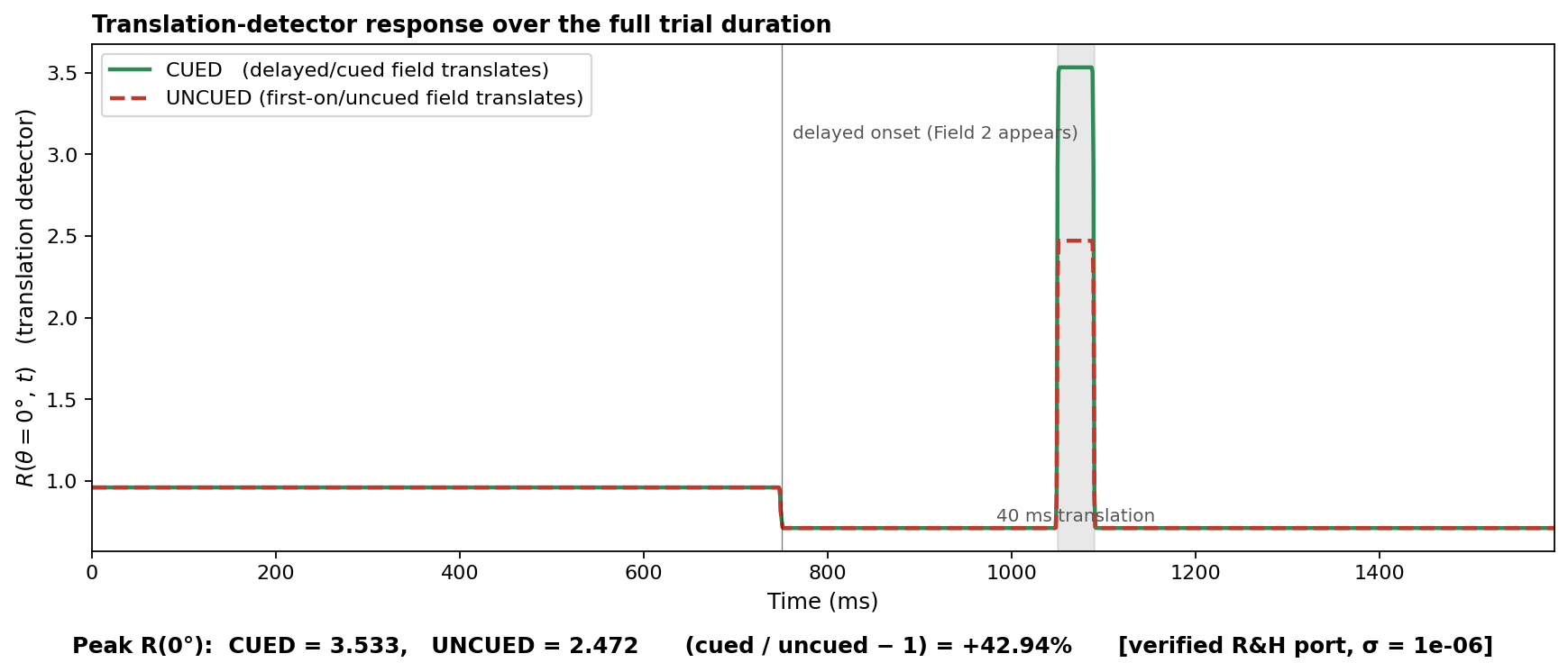
Figure 7. Attention reproduces the cued advantage. The translation-detector output R(θ = 0°, t) — the population response at the translation direction — across the whole trial, for CUED (green) and UNCUED (red), computed with the verified R&H port. With a single fixed attentional gain favoring the cued direction and no adaptation, the normalization model peaks higher for the cued field within the shaded 40 ms translation window: CUED = 3.53 vs UNCUED = 2.47, a +43% bias (at R&H's default σ = 10⁻⁶). The competition model (Figure 5) produced this same advantage from adaptation alone — so at the level of this prediction the two accounts are interchangeable: the cueing bias can be supplied by adaptation or by attention. (The magnitude depends on the normalization constant σ; the effect is strongest in the normalization-dominated regime and shrinks as σ grows.)
Verifying the implementation. Before applying this model to our stimuli, we re-implemented R&H's published model from scratch — a Python port of the authors' own `attentionModel.m` — and checked it against their MATLAB output for every quantitative figure in the 2009 paper. All nine reproduce to machine precision — maximum relative error below 10⁻¹⁴. A comparison of our model's output with R&H's original figures can be seen on the verification page.
How the time-varying application differs from R&H's original. The model we verified above is defined over space × feature: the stimulus drive is pooled across neighbouring receptive-field positions and across orientation, and each of R&H's figures is a steady-state response to a static display. To drive it with our dynamic stimulus we substitute time for their spatial (receptive-field-centre) axis, so the maps in Figures 6–7 run over direction × time. Two consequences follow, and both matter:
(1) The normalization pool does not pool over time. We set the pooling width along the time axis to ≈ 0 (an impulse), so the suppressive drive at each instant is built only from the population at that instant — pooled over direction, not over time. Adjacent time frames do not normalize one another, whereas in R&H adjacent positions do. So R&H's spatial surround-suppression has no temporal analogue here; we keep only the cross-direction (feature) normalization.
(2) There are no normalization dynamics. R&H's responses are steady-state; we apply that steady-state solution independently at every frame, i.e. we assume the normalization settles instantaneously. There is no time constant and no temporal memory.
Is it a different model? No — it is the same model in a degenerate regime. The equations are unchanged (E = A · Eᵣₐ𝓌, I = E ⊛ kernels, R = E / (I + σ)); we have only relabelled one axis and zeroed the pooling along it. Our application therefore reduces to R&H's feature-domain normalization solved separately at each moment, with no coupling across time.
The implication is sharp. Because nothing is carried across time, the cued advantage in Figures 6–7 is produced entirely by the fixed attention field at the translation instant — not by the delayed-onset history. (When the translating field's rotation pauses during the translation, the drive removed from the suppressive pool is large if that field was attention-boosted — the cued case — and small otherwise; the onset asynchrony itself never enters the computation.) This is the contrast with the competition model, where the same advantage arises from adaptation — a genuine temporal memory of the onset asynchrony. As applied here, the normalization account reproduces the bias but does not use the timing; it requires attention to already be pointed at the cued field.
The hypercolumn / point-set model
A lattice of hypercolumns — where object-based transfer becomes a spatial claim
This section documents the full model. Simpler versions — a single hypercolumn, then a minimal pair of point-sets — will be inserted before it, so the argument can be followed one addition at a time.
Both models so far are single-site: one competition circuit, one attention field, no space and no surfaces. They can produce a cued advantage, but they cannot ask the question the experiments actually pose — how a cue delivered to one attribute of one surface spreads to the other attributes of that same surface, when the two surfaces are superimposed and share every location.
Answering that requires space. This model replaces the single site with a lattice of point-sets. Each point-set is one small patch of visual field containing a motion hypercolumn (eight directions) and a colour hypercolumn (eight hues), and — the one structural commitment that matters — those two hypercolumns share a single cooperative pool. The attentional bias is direction- and hue-specific, but it enters the pool, and the pool returns a gain to every channel at that place.
That is the whole mechanism, and it is worth being precise about what it is not. There are no surface labels anywhere in the model. The front end sums over the dots of both fields into one local direction distribution and one local hue distribution; field membership never survives into the drive. What makes the gain land on the attended surface rather than the other one is simply that a dot is one thing in one place: boosting the attended direction raises the pool where attended-surface dots happen to be, and every other attribute carried by those same dots is lifted along with it. Object-based transfer falls out of co-location, not from anything that knows about objects.
Figure 8. The model, end to end. The stimulus is two superimposed transparent dot fields in a square aperture (the model seeds and wraps in a square, which is what keeps the field stationary — a disc seeded inside a square wrap drifts, and that artifact once produced a spurious cueing effect). The fields counter-rotate; one briefly translates — the probe, always at 2.26°/s regardless of field speed. This drives a lattice of 64 point-sets (σ = 0.60°, spacing 1.5σ).
Inset: inside one point-set, a motion hypercolumn (8 directions, von Mises κ = 2) and a colour hypercolumn (8 hues on a circle with red opposite green — A and B mark the two surfaces' own hues). The stimulus has only two chromatic primaries and additive red + green is yellow, so every intermediate channel is a red–green mixture and both arcs of the circle run red → yellow → green: it is mirror-symmetric about the red–green axis, with no blue or magenta anywhere in it. Both hypercolumns feed a shared cooperative pool E (τ_E = 30 ms), and both receive back the single gain that pool produces. The attentional bias enters the pool, not the channels, which is why it cannot stay confined to the attribute that was cued.
Two different pools, easily confused. The cooperative pool E is computed per point-set and runs across attributes — it is what carries the bias and produces the shared gain, and it is the mechanism. The divisive normalizer is the opposite on both counts: it operates within attribute (motion is normalized by a motion-only pool, colour by a colour-only pool) and across space, over a local Gaussian neighbourhood of σ ≈ 1.1 receptive-field spacings — the point-set plus its immediate neighbours, neither single-point-set nor grid-wide.
MT and V4 pool the V1 motion and colour maps; three read-outs follow — the attended motion itself (primary), a colour that was never cued (transfer), and the translation probe, read as an MT opponent (right − left). Independent Poisson noise enters only at the V1→MT read-out; everything upstream is deterministic.
Results
Two measures come out of the same model runs, and they are not interchangeable. The noise-free attention index asks how much larger the response is when the surface is attended — an amplitude question. The behavioural measure adds independent Poisson spike noise at the read-out and asks how much better a right-versus-left decision becomes; it is summarised as the ratio of d′ cued to d′ uncued, which is the only quantity on the same footing as the human data (the observers do an 8-AFC direction task at 12.5% chance, so percentage-point benefits do not transfer between model and experiment).
Throughout, the human numbers are plotted as a reference, not a fit. Nothing in the model has been tuned to them.
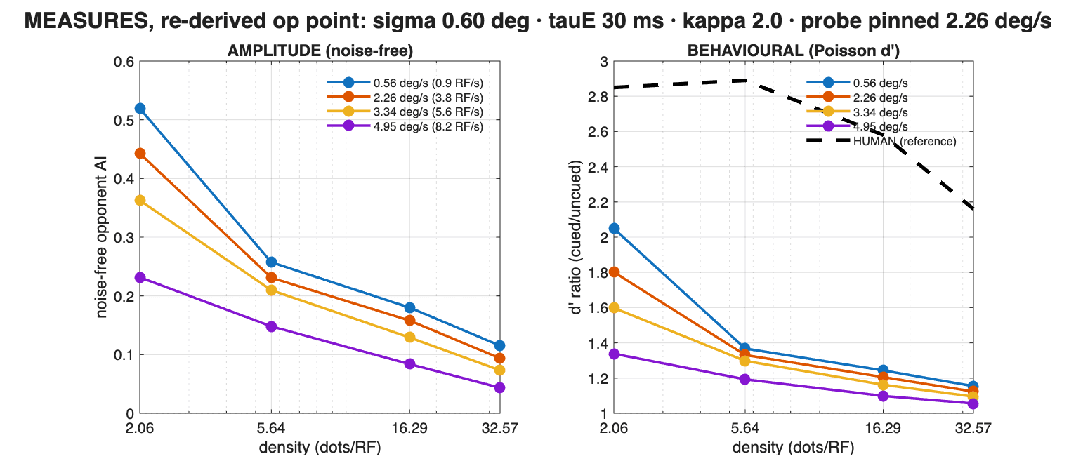
Figure 9. The two measures across the stimulus range. Density spans the human series (1.8–28.8 dots/deg², here in dots per receptive field) and field speed spans the tangential-speed distribution the rotating stimulus actually produces — from the inner edge (0.56°/s) through the area-weighted mean (3.34°/s) to the rim (4.95°/s). Left: the noise-free attention index is positive across the entire range, falling with both density and speed but never reversing. Right: the same runs read out behaviourally. The model's d′ ratio declines from 1.60 to 1.09 across the density series, against a human 2.85 → 2.16 (dashed) — the model is roughly half the human effect at the low end and, more tellingly, keeps declining where the human curve is nearly flat. The amplitude measure is healthy; the behavioural one is not. That gap is the subject of the summary below.
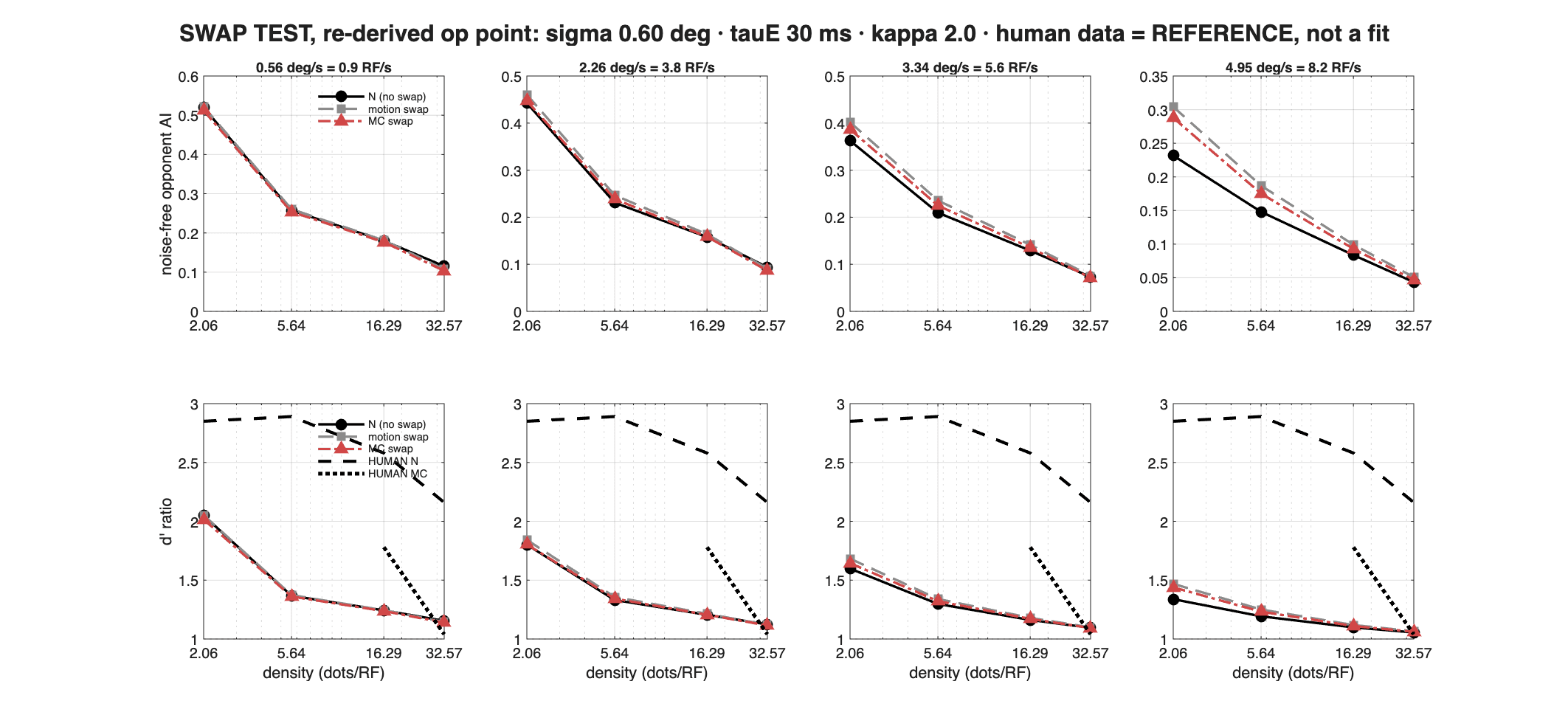
Figure 10. The feature-swap test. At the moment the probe begins, the non-translating field can reverse its motion (motion swap) and the two fields can exchange colours (MC swap) — the manipulation that asks whether the cue follows the surface or its features. Each panel is one field speed; human no-swap and MC-swap references are dashed and dotted. Two things to note. The model's MC-swap benefit tracks the no-swap condition at every density, whereas the observers lose it entirely at the highest density (1.04 versus 2.16). And the motion-swap condition sits slightly above no-swap — a known confound rather than a result: the attentional bias here is a sustained feature preference, so when a field adopts the attended direction at probe onset it refreshes the cued pool. Reproducing the density × swap interaction remains the model's outstanding failure.
Watch the model run
Figure 11. Watch it run. Real model output, not an illustration — every panel is exported directly from the simulation at the operating point above, and the chain reads left to right exactly as it does in the model. Stimulus: the actual dots, in the square aperture, red field against green field, with the rightward probe marked when it fires. Stimulus drive: how strongly the dots drive each of the 64 point-sets — identical for cued and uncued, because the cue has not acted yet. This is the raw drive, shown before the model's per-point-set input normalization; that normalization divides each point-set's drive by its own total, so after it the map is uniform by construction. The lattice maps are deliberately grayscale, so map intensity is never confused with the dot colours or the hue rosette. Cooperative pool: the same lattice for the two attentional states; this is where the cue lives, and the difference between these two maps is the effect. MT / V4: the pooled read-outs as 8-channel rosettes, motion and colour, cued beside uncued.
Below, the three attention indices through the trial, with the pre-probe and probe windows shaded. Watch the primary and colour indices build together during viewing — they land on top of each other to three decimals, and that equality is the transfer: one shared gain lifting the attended surface's motion and its colour alike. Note both indices compare the same channel between the cued and uncued runs (DOWN for motion, GREEN for colour); what differs between the runs is only whether that surface is attended — while the translation index appears only when the probe arrives. Then push the density up and the speed up: the two pool maps become progressively harder to tell apart, and the indices collapse with them. That is what the failure looks like from the inside.
These panels run a single dot layout, as the MATLAB viewer does, so the traces are noisier than the multi-layout averages in Figures 9 and 10; the 8-layout probe mean is quoted alongside for comparison.
What the model shows
The mechanism works, and it works for the reason we wanted it to. A bias applied to one attribute, entering a pool shared across attributes at a place, transfers to the other attributes of the same surface — with no object label anywhere in the model. Attending a direction lifts a colour that was never cued, because the dots carrying both are in the same receptive fields.
Spatial scale turned out to be the binding constraint, and it is not a free parameter. The gain lives in the pool, which is a map over places, while the surfaces move. Sweeping speed to the point of failure shows the effect dies once a dot travels about 1.3 receptive-field sigmas during the interval the pool has to bridge — the same constant for every RF size tested. That gives a hard ceiling,
v_crit ≈ 1.3 σ / (τ_E + probe duration),
which is ~9.8°/s at the current settings. The rim of the human stimulus sits at about half of it, which is why σ = 0.60° works and σ = 0.30° does not; at the smaller size the index actually reverses inside the range the observers were tested in. Enlarging the receptive field or lengthening the pool's time constant moves this ceiling. Nothing in the present architecture removes it.
The amplitude is right and the behaviour is not. The noise-free index is positive across the whole stimulus range, but the behavioural d′ ratio reaches only ~1.6 where observers show ~2.9, and it keeps falling where the human curve is flat. Two things follow, and both are quantitative rather than matters of taste. Under independent Poisson noise with a gain mechanism, d′ scales as the square root of response, so the d′ ratio is roughly the square root of the response ratio — which means matching the human effect by response gain alone would need an ~8× enhancement of firing rate. Attentional rate modulation in visual cortex is tens of percent. And pooling more neurons cannot rescue it either, because recruitment raises cued and uncued alike and leaves their ratio untouched. Recruitment can explain why performance does not collapse; it cannot explain how large the effect is.
So the model is not short of gain — it is using gain to do a job that selection does better. That, rather than any parameter, is what the next round should test.
Where it goes next
Four directions, roughly in order of cost:
- – Separate the sampling density from the receptive-field size. The lattice currently tiles at 1.5σ, so enlarging the RF to fix the speed limit cut the population from 256 point-sets to 64 — and with it a factor of two in pooled sensitivity. Cortex oversamples heavily; RFs overlap. Sampling the same σ = 0.60° field at a finer spacing recovers that loss for free, since each unit still carries independent spiking noise.
- – Give density something to buy. The input normalization is currently almost perfectly scale-invariant, so a receptive field holding thirty dots produces the same drive as one holding three, and more dots therefore yield no more spikes. Restoring a genuine semi-saturation constant — standard for V1 normalization — lets drive grow sub-linearly with density, which is the only way recruitment can help at all.
- – Let attention weight the read-out, not just the response. The pool is already surface-specific; at present it is used only to scale responses. Using it to weight which point-sets contribute to the decision would improve sensitivity by excluding uninformative units, which is far more efficient than amplifying signal — and it is the standard resolution of why behavioural attention effects so exceed single-neuron rate modulations. This is the one change with the leverage to close the magnitude gap.
- – Let the gain field move with the surface. Advecting the pool by the locally decoded velocity would remove the speed ceiling rather than merely relocating it, and it is well motivated by predictive remapping. It also makes an interesting prediction: at high density the local velocity estimate is contaminated by the other surface, so the tracking should degrade with crowding — which is the shape of the density × swap interaction the model currently fails to produce.
Further out, the honest limitation is the front end. Each dot's direction and colour are handed to the model as ground truth, so segregation can never actually fail. Computing motion from the rendered image would make direction an inference, with false correspondences between surfaces — the point at which crowding could break surface identity on its own, rather than merely diluting it.